Which Of The Following Situations Allows For Data Not To Be Lost In A Raid Array?

Any of a set of standard configurations of Redundant Arrays of Independent Disks

In computer storage, the standard RAID levels comprise a basic set of RAID ("redundant array of independent disks" or "redundant array of inexpensive disks") configurations that apply the techniques of striping, mirroring, or parity to create big reliable data stores from multiple full general-purpose computer hd drives (HDDs). The nigh mutual types are RAID 0 (striping), RAID one (mirroring) and its variants, RAID 5 (distributed parity), and RAID 6 (dual parity). Multiple RAID levels can also be combined or nested, for instance RAID 10 (striping of mirrors) or RAID 01 (mirroring stripe sets). RAID levels and their associated data formats are standardized by the Storage Networking Manufacture Clan (SNIA) in the Common RAID Disk Drive Format (DDF) standard.^[one] The numerical values merely serve as identifiers and exercise not signify performance, reliability, generation, or whatever other metric.

While almost RAID levels tin provide proficient protection against and recovery from hardware defects or lacking sectors/read errors (hard errors), they do non provide whatever protection confronting data loss due to catastrophic failures (fire, water) or soft errors such as user error, software malfunction, or malware infection. For valuable data, RAID is merely ane building block of a larger data loss prevention and recovery scheme – it cannot replace a backup plan.

RAID 0 [edit]

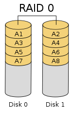
Diagram of a RAID 0 setup

RAID 0 (too known as a stripe set or striped volume) splits ("stripes") data evenly across two or more disks, without parity information, redundancy, or fault tolerance. Since RAID 0 provides no error tolerance or redundancy, the failure of one drive will cause the entire array to fail; every bit a result of having data striped across all disks, the failure volition upshot in total information loss. This configuration is typically implemented having speed as the intended goal.^{[ii] [3]} RAID 0 is normally used to increase performance, although information technology can also be used as a way to create a big logical volume out of two or more physical disks.^[4]

A RAID 0 setup can be created with disks of differing sizes, but the storage space added to the array past each disk is express to the size of the smallest disk. For example, if a 120 GB disk is striped together with a 320 GB disk, the size of the array will be 120 GB × ii = 240 GB. However, some RAID implementations allow the remaining 200 GB to exist used for other purposes.

The diagram in this section shows how the data is distributed into stripes on two disks, with A1:A2 as the first stripe, A3:A4 as the second one, etc. Once the stripe size is defined during the creation of a RAID 0 array, it needs to exist maintained at all times. Since the stripes are accessed in parallel, an north-bulldoze RAID 0 array appears as a single large disk with a data rate due north times college than the unmarried-disk rate.

Functioning [edit]

A RAID 0 array of due north drives provides data read and write transfer rates upwards to n times equally high equally the individual drive rates, but with no data back-up. Equally a result, RAID 0 is primarily used in applications that require high operation and are able to tolerate lower reliability, such every bit in scientific computing^[v] or computer gaming.^{[half dozen]}

Some benchmarks of desktop applications show RAID 0 performance to exist marginally better than a single drive.^{[7] [viii]} Some other article examined these claims and ended that "striping does non ever increment performance (in sure situations it will actually exist slower than a non-RAID setup), just in nearly situations it will yield a significant comeback in functioning".^{[9] [10]} Constructed benchmarks show unlike levels of performance improvements when multiple HDDs or SSDs are used in a RAID 0 setup, compared with single-drive performance. However, some synthetic benchmarks also show a drop in performance for the aforementioned comparison.^{[11] [12]}

RAID ane [edit]

Diagram of a RAID 1 setup

RAID ane consists of an exact copy (or mirror) of a ready of data on two or more than disks; a classic RAID 1 mirrored pair contains 2 disks. This configuration offers no parity, striping, or spanning of disk infinite across multiple disks, since the data is mirrored on all disks belonging to the array, and the array tin can only be equally big as the smallest member deejay. This layout is useful when read performance or reliability is more of import than write performance or the resulting data storage capacity.^{[13] [14]}

The assortment will continue to operate so long equally at least one member drive is operational.^[xv]

Operation [edit]

Whatsoever read request tin can be serviced and handled by any drive in the array; thus, depending on the nature of I/O load, random read performance of a RAID i array may equal upwardly to the sum of each fellow member's functioning,^[a] while the write performance remains at the level of a single disk. However, if disks with different speeds are used in a RAID 1 assortment, overall write performance is equal to the speed of the slowest disk.^{[14] [xv]}

Synthetic benchmarks show varying levels of performance improvements when multiple HDDs or SSDs are used in a RAID one setup, compared with single-bulldoze performance. However, some constructed benchmarks also show a drop in performance for the same comparison.^{[11] [12]}

RAID 2 [edit]

Diagram of a RAID 2 setup

RAID ii, which is rarely used in exercise, stripes data at the bit (rather than block) level, and uses a Hamming lawmaking for error correction. The disks are synchronized past the controller to spin at the same angular orientation (they accomplish index at the same time^[16]), and then information technology mostly cannot service multiple requests simultaneously.^{[17] [18]} Nonetheless, depending with a high rate Hamming code, many spindles would operate in parallel to simultaneously transfer data so that "very loftier information transfer rates" are possible^[19] every bit for instance in the DataVault where 32 data $.25 were transmitted simultaneously.

With all hd drives implementing internal error correction, the complexity of an external Hamming code offered niggling advantage over parity and so RAID ii has been rarely implemented; information technology is the simply original level of RAID that is not currently used.^{[17] [18]}

RAID iii [edit]

Diagram of a RAID iii setup of vi-byte blocks and 2 parity bytes, shown are two blocks of data in dissimilar colors.

RAID 3, which is rarely used in practice, consists of byte-level striping with a defended parity deejay. One of the characteristics of RAID iii is that information technology more often than not cannot service multiple requests simultaneously, which happens because whatever single cake of data will, by definition, be spread across all members of the set and will reside in the same physical location on each disk. Therefore, whatsoever I/O performance requires activity on every disk and unremarkably requires synchronized spindles.

This makes information technology suitable for applications that demand the highest transfer rates in long sequential reads and writes, for example uncompressed video editing. Applications that make small-scale reads and writes from random disk locations volition get the worst operation out of this level.^[eighteen]

The requirement that all disks spin synchronously (in a lockstep) added design considerations that provided no meaning advantages over other RAID levels. Both RAID iii and RAID 4 were quickly replaced by RAID 5.^[xx] RAID 3 was unremarkably implemented in hardware, and the performance issues were addressed by using big deejay caches.^[eighteen]

RAID 4 [edit]

Diagram 1: A RAID four setup with dedicated parity disk with each color representing the group of blocks in the respective parity block (a stripe)

RAID 4 consists of cake-level striping with a dedicated parity disk. As a consequence of its layout, RAID four provides practiced performance of random reads, while the performance of random writes is low due to the need to write all parity data to a unmarried disk,^[21] unless the filesystem is RAID-iv-aware and compensates for that.

An advantage of RAID 4 is that it can be quickly extended online, without parity recomputation, as long as the newly added disks are completely filled with 0-bytes.

In diagram 1, a read request for cake A1 would be serviced past deejay 0. A simultaneous read asking for block B1 would have to wait, merely a read request for B2 could be serviced concurrently past disk 1.

RAID five [edit]

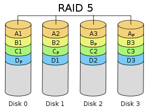
Diagram of a RAID v layout with each color representing the grouping of data blocks and associated parity block (a stripe). This diagram shows Left Asynchronous layout

RAID v consists of block-level striping with distributed parity. Unlike in RAID 4, parity information is distributed amidst the drives. Information technology requires that all drives just 1 be present to operate. Upon failure of a unmarried drive, subsequent reads can be calculated from the distributed parity such that no data is lost.^[v] RAID 5 requires at least three disks.^[22]

In that location are many layouts of data and parity in a RAID 5 disk drive array depending upon the sequence of writing across the disks,^[23] that is:

1. the sequence of data blocks written, left to correct or right to left on the disk assortment, of disks 0 to N, and
2. the location of the parity block at the starting time or end of the stripe, and
3. the location of the first block of a stripe with respect to parity of the previous stripe.

The effigy to the right shows 1) data blocks written left to right, 2) the parity block at the end of the stripe and 3) the first block of the next stripe non on the aforementioned deejay as the parity block of the previous stripe. It can be designated as a Left Asynchronous RAID 5 layout^[23] and this is the but layout identified in the last edition of The Raid Volume ^[24] published by the defunct Raid Advisory Board. ^[25] In a Synchronous layout the data showtime cake of the next stripe is written on the same drive equally the parity cake of the previous stripe.

In comparison to RAID four, RAID five'south distributed parity evens out the stress of a dedicated parity disk among all RAID members. Additionally, write performance is increased since all RAID members participate in the serving of write requests. Although it will not be as efficient as a striping (RAID 0) setup, because parity must still exist written, this is no longer a bottleneck.^[26]

Since parity adding is performed on the full stripe, modest changes to the array experience write amplification ^{[ citation needed ]}: in the worst instance when a single, logical sector is to be written, the original sector and the according parity sector need to exist read, the original information is removed from the parity, the new data calculated into the parity and both the new data sector and the new parity sector are written.

RAID half dozen [edit]

Diagram of a RAID 6 setup, which is identical to RAID 5 other than the addition of a second parity cake

RAID six extends RAID five past adding another parity block; thus, it uses block-level striping with two parity blocks distributed across all fellow member disks.^[27]

As in RAID five, in that location are many layouts of RAID 6 disk arrays depending upon the direction the information blocks are written, the location of the parity blocks with respect to the information blocks and whether or not the kickoff data block of a subsequent stripe is written to the same drive as the concluding parity block of the prior stripe. The figure to the right is just ane of many such layouts.

Co-ordinate to the Storage Networking Industry Association (SNIA), the definition of RAID 6 is: "Whatsoever form of RAID that can go along to execute read and write requests to all of a RAID array's virtual disks in the presence of any two concurrent disk failures. Several methods, including dual check information computations (parity and Reed–Solomon), orthogonal dual parity check data and diagonal parity, have been used to implement RAID Level six."^[28]

Performance [edit]

RAID 6 does non take a functioning punishment for read operations, only it does have a functioning penalty on write operations considering of the overhead associated with parity calculations. Performance varies greatly depending on how RAID 6 is implemented in the manufacturer's storage architecture—in software, firmware, or past using firmware and specialized ASICs for intensive parity calculations. RAID 6 tin read upward to the same speed every bit RAID 5 with the aforementioned number of physical drives.^[29]

When either diagonal or orthogonal dual parity is used, a second parity calculation is necessary for write operations. This doubles CPU overhead for RAID-six writes, versus single-parity RAID levels. When a Reed Solomon code is used, the second parity calculation is unnecessary. Reed Solomon has the advantage of allowing all redundancy data to exist contained inside a given stripe.

Simplified parity example [edit]

Suppose nosotros would like to distribute our data over ${\displaystyle n}$ chunks. Our goal is to define 2 parity values ${\displaystyle \mathbf {P} }$ and ${\displaystyle \mathbf {Q} }$ , known as syndromes, resulting in a organisation of ${\displaystyle n+2}$ physical drives that is resilient to the loss of any two of them. In social club to generate more than a single independent syndrome, we volition need to perform our parity calculations on information chunks of size ${\displaystyle k>i.}$ A typical choice in practice is a chunk size ${\displaystyle k=8}$ , i.e. striping the data per-byte. We will denote the base-ii representation of a data clamper ${\displaystyle D}$ equally ${\displaystyle d_{0}d_{one}...d_{k-1}}$ , where each ${\displaystyle d_{i}}$ is either 0 or 1.

If we are using a modest number of chunks ${\displaystyle north\leq g}$ , we tin utilize a uncomplicated parity computation, which will help motivate the apply of the Reed–Solomon organization in the general instance. For our first parity value ${\displaystyle \mathbf {P} }$ , nosotros compute the uncomplicated XOR of the information across the stripes, every bit with RAID 5. This is written

$${\displaystyle \mathbf {P} =D_{0}\;\oplus \;D_{1}\;\oplus \;D_{2}\;\oplus \;...\;\oplus \;D_{due north-1}}$$

where ${\displaystyle \oplus }$ denotes the XOR operator. The second parity value is analogous, but with each data chunk flake-shifted a different amount. Writing ${\displaystyle \mathrm {shift} (D)=d_{1}...d_{thou-1}d_{0}}$ , we define

$${\displaystyle \mathbf {Q} =D_{0}\oplus \mathrm {shift} (D_{1})\oplus \mathrm {shift} ^{2}(D_{two})\oplus ...\oplus \mathrm {shift} ^{n-ane}(D_{northward-1})}$$

In the effect of a single drive failure, the data can be recomputed from ${\displaystyle \mathbf {P} }$ just like with RAID 5. We will show we can also recover from simultaneous failure of two drives. If we lose a data chunk and ${\displaystyle \mathbf {P} }$ , we can recover from ${\displaystyle \mathbf {Q} }$ and the remaining information past using the fact that ${\displaystyle D\oplus D=0}$ . Suppose on a arrangement of ${\displaystyle n=4}$ chunks, the drive containing chunk ${\displaystyle D_{three}}$ has failed. We tin compute

$${\displaystyle \mathbf {Q} \oplus D_{0}\oplus \mathrm {shift} (D_{1})\oplus \mathrm {shift} ^{2}(D_{2})=\mathrm {shift} ^{three}(D_{iii})}$$

and recover the lost data ${\displaystyle D_{three}}$ by undoing the chip shift. We tin can also recover from the failure of 2 information disks by computing the XOR of ${\displaystyle \mathbf {P} }$ and ${\displaystyle \mathbf {Q} }$ with the remaining information. If in the previous case, chunk ${\displaystyle D_{0}}$ had been lost as well, we would compute

$${\displaystyle A=\mathbf {P} \oplus D_{1}\oplus D_{ii}=D_{0}\oplus D_{3}}$$

$${\displaystyle B=\mathbf {Q} \oplus \mathrm {shift} (D_{1})\oplus \mathrm {shift} ^{ii}(D_{2})=D_{0}\oplus \mathrm {shift} ^{3}(D_{3})}$$

On a bitwise level, this represents a system of ${\displaystyle 2k}$ equations in ${\displaystyle 2k}$ unknowns which uniquely determine the lost data.

This system will no longer work practical to a larger number of drives ${\displaystyle n>g}$ . This is because if we repeatedly use the shift operator ${\displaystyle k}$ times to a chunk of length ${\displaystyle chiliad}$ , we end up back where we started. If we tried to apply the algorithm above to a system containing ${\displaystyle yard}$ data disks, the right-mitt side of the second equation would be ${\displaystyle D_{0}\oplus \mathrm {shift} ^{k}(D_{k})=D_{0}\oplus D_{chiliad}}$ , which is the aforementioned as the first set up of equations. This would only yield one-half as many equations as needed to solve for the missing values.

General parity system [edit]

It is possible to support a far greater number of drives past choosing the parity function more advisedly. The upshot we confront is to ensure that a system of equations over the finite field ${\displaystyle \mathbb {Z} _{2}}$ has a unique solution, so we will plow to the theory of polynomial equations. Consider the Galois field ${\displaystyle GF(thou)}$ with ${\displaystyle 1000=2^{g}}$ . This field is isomorphic to a polynomial field ${\displaystyle F_{2}[x]/(p(10))}$ for a suitable irreducible polynomial ${\displaystyle p(x)}$ of degree ${\displaystyle k}$ over ${\displaystyle \mathbb {Z} _{two}}$ . We will represent the data elements ${\displaystyle D}$ equally polynomials ${\displaystyle \mathbf {D} =d_{k-i}10^{k-ane}+d_{k-ii}10^{thousand-2}+...+d_{one}ten+d_{0}}$ in the Galois field. Let ${\displaystyle \mathbf {D} _{0},...,\mathbf {D} _{n-1}\in GF(chiliad)}$ stand for to the stripes of information across hard drives encoded as field elements in this manner. We will use ${\displaystyle \oplus }$ to denote addition in the field, and concatenation to denote multiplication. The reuse of ${\displaystyle \oplus }$ is intentional: this is considering addition in the finite field ${\displaystyle \mathbb {Z} _{ii}}$ represents to the XOR operator, and so computing the sum of two elements is equivalent to computing XOR on the polynomial coefficients.

A generator of a field is an element of the field such that ${\displaystyle g^{i}}$ is unlike for each non-negative ${\displaystyle i<m-1}$ . This means each chemical element of the field, except the value ${\displaystyle 0}$ , can be written every bit a ability of ${\displaystyle g.}$ A finite field is guaranteed to have at to the lowest degree one generator. Pick one such generator ${\displaystyle g}$ , and define ${\displaystyle \mathbf {P} }$ and ${\displaystyle \mathbf {Q} }$ as follows:

${\displaystyle \mathbf {P} =\bigoplus _{i}{\mathbf {D} _{i}}=\mathbf {D} _{0}\;\oplus \;\mathbf {D} _{1}\;\oplus \;\mathbf {D} _{2}\;\oplus \;...\;\oplus \;\mathbf {D} _{due north-i}}$

${\displaystyle \mathbf {Q} =\bigoplus _{i}{yard^{i}\mathbf {D} _{i}}=g^{0}\mathbf {D} _{0}\;\oplus \;m^{1}\mathbf {D} _{1}\;\oplus \;g^{2}\mathbf {D} _{ii}\;\oplus \;...\;\oplus \;g^{due north-1}\mathbf {D} _{n-ane}}$

As before, the offset checksum ${\displaystyle \mathbf {P} }$ is only the XOR of each stripe, though interpreted at present as a polynomial. The issue of ${\displaystyle g^{i}}$ can be thought of as the action of a carefully called linear feedback shift register on the information chunk.^[xxx] Unlike the bit shift in the simplified instance, which could only be applied ${\displaystyle grand}$ times before the encoding began to repeat, applying the operator ${\displaystyle g}$ multiple times is guaranteed to produce ${\displaystyle m=ii^{thou}-1}$ unique invertible functions, which will allow a clamper length of ${\displaystyle k}$ to support upwards to ${\displaystyle 2^{k}-1}$ data pieces.

If one data chunk is lost, the situation is similar to the one before. In the case of two lost data chunks, we can compute the recovery formulas algebraically. Suppose that ${\displaystyle \mathbf {D} _{i}}$ and ${\displaystyle \mathbf {D} _{j}}$ are the lost values with ${\displaystyle i\neq j}$ , then, using the other values of ${\displaystyle D}$ , nosotros find constants ${\displaystyle A}$ and ${\displaystyle B}$ :

${\displaystyle A=\mathbf {P} \;\oplus \;(\bigoplus _{\ell :\;\ell \not =i\;\mathrm {and} \;\ell \not =j}{D_{\ell }})=D_{i}\oplus D_{j}}$

${\displaystyle B=\mathbf {Q} \;\oplus \;(\bigoplus _{\ell :\;\ell \not =i\;\mathrm {and} \;\ell \not =j}{g^{\ell }D_{\ell }})=one thousand^{i}D_{i}\oplus g^{j}D_{j}}$

We tin can solve for ${\displaystyle D_{i}}$ in the 2nd equation and plug it into the first to find ${\displaystyle D_{j}=(g^{thousand-i+j}\oplus one)^{-one}(g^{g-i}B\oplus A)}$ , and then ${\displaystyle D_{i}=A\oplus D_{j}}$ .

Unlike P, The ciphering of Q is relatively CPU intensive, every bit it involves polynomial multiplication in ${\displaystyle F_{2}[x]/(p(x))}$ . This can be mitigated with a hardware implementation or by using an FPGA.

Comparison [edit]

The following table provides an overview of some considerations for standard RAID levels. In each case, array space efficiency is given as an expression in terms of the number of drives, n; this expression designates a partial value between zero and one, representing the fraction of the sum of the drives' capacities that is available for use. For example, if three drives are arranged in RAID iii, this gives an array space efficiency of 1 − 1/n = ane − ane/3 = 2/3 ≈ 67%; thus, if each drive in this example has a capacity of 250 GB, then the array has a total capacity of 750 GB but the capacity that is usable for information storage is only 500 GB.

Level	Description	Minimum number of drives[b]	Space efficiency	Fault tolerance	Read functioning	Write performance
					as factor of unmarried deejay
RAID 0	Block-level striping without parity or mirroring	ii	1	None	n	n
RAID 1	Mirroring without parity or striping	2	1 / n	n − one drive failures	n [a] [15]	1 [c] [xv]
RAID two	Bit-level striping with Hamming lawmaking for mistake correction	three	1 − one / n log2 (n + one)	1 bulldoze failure[d]	Depends	Depends
RAID three	Byte-level striping with dedicated parity	3	1 − 1 / n	Ane drive failure	n − one	n − 1 [e]
RAID four	Block-level striping with dedicated parity	3	i − 1 / northward	One drive failure	n − 1	n − i [e] [ citation needed ]
RAID five	Cake-level striping with distributed parity	3	1 − 1 / due north	One drive failure	north [east]	unmarried sector: ane / four full stripe: n − 1 [e] [ citation needed ]
RAID six	Cake-level striping with double distributed parity	iv	i − ii / n	Two bulldoze failures	n [due east]	unmarried sector: ane / 6 full stripe: due north − 2 [e] [ commendation needed ]

System implications [edit]

In measurement of the I/O performance of five filesystems with five storage configurations—single SSD, RAID 0, RAID one, RAID 10, and RAID 5 it was shown that F2FS on RAID 0 and RAID 5 with 8 SSDs outperforms EXT4 by 5 times and fifty times, respectively. The measurements too suggest that the RAID controller can be a significant bottleneck in edifice a RAID system with high speed SSDs.^[31]

Nested RAID [edit]

Combinations of two or more standard RAID levels. They are also known equally RAID 0+ane or RAID 01, RAID 0+3 or RAID 03, RAID 1+0 or RAID 10, RAID five+0 or RAID fifty, RAID 6+0 or RAID 60, and RAID ten+0 or RAID 100.

Not-standard variants [edit]

In addition to standard and nested RAID levels, alternatives include not-standard RAID levels, and non-RAID drive architectures. Non-RAID bulldoze architectures are referred to past like terms and acronyms, notably JBOD ("just a bunch of disks"), SPAN/BIG, and MAID ("massive array of idle disks").

Notes [edit]

1. ^ ^{a b} Theoretical maximum, every bit low as single-disk performance in do
2. ^ Assumes a non-degenerate minimum number of drives
3. ^ If disks with unlike speeds are used in a RAID 1 array, overall write performance is equal to the speed of the slowest deejay.
4. ^ RAID 2 can recover from one bulldoze failure or repair corrupt data or parity when a corrupted bit's corresponding data and parity are skilful.
5. ^ ^{a b c d e f} Assumes hardware capable of performing associated calculations fast plenty

References [edit]

1. ^ "Mutual raid Disk Data Format (DDF)". SNIA.org. Storage Networking Industry Association. Retrieved 2013-04-23 .
2. ^ "RAID 0 Data Recovery". DataRecovery.net . Retrieved 2015-04-30 .
3. ^ "Understanding RAID". CRU-Inc.com . Retrieved 2015-04-30 .
4. ^ "How to Combine Multiple Hard Drives Into Ane Volume for Cheap, High-Chapters Storage". LifeHacker.com. 2013-02-26. Retrieved 2015-04-thirty .
5. ^ ^{a b} Chen, Peter; Lee, Edward; Gibson, Garth; Katz, Randy; Patterson, David (1994). "RAID: High-Operation, Reliable Secondary Storage". ACM Calculating Surveys. 26 (2): 145–185. CiteSeerX10.1.i.41.3889. doi:10.1145/176979.176981. S2CID 207178693.
6. ^ de Kooter, Sebastiaan (2015-04-13). "Gaming storage shootout 2015: SSD, HDD or RAID 0, which is best?". GamePlayInside.com . Retrieved 2015-09-22 .
7. ^ "Western Digital'southward Raptors in RAID-0: Are two drives better than one?". AnandTech.com. AnandTech. July 1, 2004. Retrieved 2007-xi-24 .
8. ^ "Hitachi Deskstar 7K1000: Two Terabyte RAID Redux". AnandTech.com. AnandTech. April 23, 2007. Retrieved 2007-xi-24 .
9. ^ "RAID 0: Hype or blessing?". Tweakers.net. Persgroep Online Services. August 7, 2004. Retrieved 2008-07-23 .
10. ^ "Does RAID0 Really Increase Disk Performance?". HardwareSecrets.com. November ane, 2006.
11. ^ ^{a b} Larabel, Michael (2014-ten-22). "Btrfs RAID HDD Testing on Ubuntu Linux 14.x". Phoronix. Retrieved 2015-09-19 .
12. ^ ^{a b} Larabel, Michael (2014-x-29). "Btrfs on 4 × Intel SSDs In RAID 0/one/5/six/10". Phoronix. Retrieved 2015-09-nineteen .
13. ^ "FreeBSD Handbook: 19.3. RAID 1 – Mirroring". FreeBSD.org. 2014-03-23. Retrieved 2014-06-11 .
14. ^ ^{a b} "Which RAID Level is Right for Me?: RAID 1 (Mirroring)". Adaptec.com. Adaptec. Retrieved 2014-01-02 .
15. ^ ^{a b c d} "Selecting the Best RAID Level: RAID 1 Arrays (Sun StorageTek SAS RAID HBA Installation Guide)". Docs.Oracle.com. Oracle Corporation. 2010-12-23. Retrieved 2014-01-02 .
16. ^ "RAID 2". Techopedia. Techopedia. Retrieved 11 Dec 2019.
17. ^ ^{a b} Vadala, Derek (2003). Managing RAID on Linux. O'Reilly Series (illustrated ed.). O'Reilly. p. 6. ISBN9781565927308.
18. ^ ^{a b c d} Marcus, Evan; Stern, Hal (2003). Blueprints for high availability (2, illustrated ed.). John Wiley and Sons. p. 167. ISBN9780471430261.
19. ^ The RAIDbook, 4th Edition, The RAID Informational Board, June 1995, p.101
20. ^ Meyers, Michael; Jernigan, Scott (2003). Mike Meyers' A+ Guide to Managing and Troubleshooting PCs (illustrated ed.). McGraw-Colina Professional. p. 321. ISBN9780072231465.
21. ^ Natarajan, Ramesh (2011-11-21). "RAID 2, RAID three, RAID iv and RAID 6 Explained with Diagrams". TheGeekStuff.com . Retrieved 2015-01-02 .
22. ^ "RAID 5 Data Recovery FAQ". VantageTech.com. Vantage Technologies. Retrieved 2014-07-sixteen .
23. ^ ^{a b} "RAID Data - Linux RAID-5 Algorithms". Ashford calculator Consulting Service . Retrieved February sixteen, 2021.
24. ^ Massigilia, Paul (February 1997). The RAID Volume, 6th Edition. RAID Advisory Board. pp. 101–129.
25. ^ "Welcome to the RAID Advisory Lath". RAID Advisory Lath. April 6, 2001. Archived from the original on 2001-04-06. Retrieved February 16, 2021. Last valid archived webpage at Wayback Machine}}
26. ^ Koren, State of israel. "Basic RAID Organizations". ECS.UMass.edu. Academy of Massachusetts. Retrieved 2014-xi-04 .
27. ^ "Sun StorageTek SAS RAID HBA Installation Guide, Appendix F: Selecting the Best RAID Level: RAID 6 Arrays". Docs.Oracle.com. 2010-12-23. Retrieved 2015-08-27 .
28. ^ "Lexicon R". SNIA.org. Storage Networking Industry Association. Retrieved 2007-11-24 .
29. ^ Faith, Rickard Eastward. (13 May 2009). "A Comparison of Software RAID Types".
30. ^ Anvin, H. Peter (May 21, 2009). "The Mathematics of RAID-6" (PDF). Kernel.org. Linux Kernel System. Retrieved November four, 2009.
31. ^ Park, Chanhyun; Lee, Seongjin; Won, Youjip (2014). An Analysis on Empirical Operation of SSD-Based RAID. Information Sciences and Systems. Vol. 2014. pp. 395–405. doi:10.1007/978-three-319-09465-6_41. ISBN978-iii-319-09464-9.

Further reading [edit]

• "Learning About RAID". Support.Dell.com. Dell. 2009. Archived from the original on 2009-02-twenty. Retrieved 2016-04-15 .
• Redundant Arrays of Inexpensive Disks (RAIDs), affiliate 38 from the Operating Systems: Three Like shooting fish in a barrel Pieces book by Remzi H. Arpaci-Dusseau and Andrea C. Arpaci-Dusseau

External links [edit]

• IBM summary on RAID levels
• RAID 5 parity explanation and checking tool
• RAID Calculator for Standard RAID Levels and Other RAID Tools
• Sun StorEdge 3000 Family unit Configuration Service two.5 User'south Guide: RAID Basics

Which Of The Following Situations Allows For Data Not To Be Lost In A Raid Array?,

Source: https://en.wikipedia.org/wiki/Standard_RAID_levels

Posted by: gillhited1992.blogspot.com

Share this post